Differential Evolution with Competitive Control-parameter Setting
Contents
Problem Specification
The global optimization problem with box (boundary) constraints is formed as follows:
For a given objective function f: D \rightarrow {\mathbb R}, \ D \subset {\mathbb R}^{d}
the point {\mathbf x}^{*} is to be found such that \forall \vec{x} \in D \ f(\vec{x}^{*}) \leq f(\vec{x}).
The point \vec{x}^{*} is called the global minimum, D is the search space defined as d- dimensional box, D=\prod_{i=1}^{d} [a_i,b_i], a_i < b_i, i=1,2,\ldots,d.
The problem of the global optimization is hard and plenty of stochastic algorithms were proposed for its solution, see e.g. [1]. The authors of many such stochastic algorithms claim the efficiency and the reliability of searching for the global minimum. The reliability means that the point with minimal function value found in the search process is sufficiently close to the global minimum point and the efficiency means that the algorithm finds a point sufficiently close to the global minimum point at reasonable time. However, when we use such algorithms, we face the problem of the setting their control parameters. The efficiency and the reliability of many algorithms is strongly dependent on the values of control parameters. Recommendations given by authors are often vague or uncertain. A user is supposed to be able to change the parameter values according to the results of trial-and-error preliminary experiments with the search process. Such attempt is not acceptable in tasks, where the global optimization is one step on the way to the solution of the user’s problem or when the user has no experience in fine art of control parameter tuning. Adaptive robust algorithms reliable enough at reasonable time-consumption without the necessity of fine tuning their input parameters have been studied in recent years.
The differential evolution (DE) [7] has become one of the most popular algorithms for the continuous global optimization problems in last decade years, see [6]. However, it is known that the efficiency of the search for the global minimum is very sensitive to the setting of its control parameters. That is why the self-adaptive DE was proposed and included into this library. Recent state of adaptive parameter control in differential evolution is summarized in [2], [4], [5].
Description of Implemented Algorithms
The differential evolution is population-based algorithm which works with two generations P and Q of the same size N. A new trial point \vec{y} is composed of the current point \vec{x}_i of old generation and the point \vec{u} obtained by using mutation. If f(\vec{y})<f(\vec{x}_i) the point \vec{y} is inserted into the new generation Q instead of \vec{x}_i. After completion of the new generation Q the old generation P is replaced by Q and the search continues until stopping condition is fulfilled. The DE algorithm can be written as follows:
Algorithm 1: DE Algorithm
1 2 3 4 5 6 7 8 9 10 11 12 | generate P = (x[1], x[2], ..., x[N]); // N points in D
repeat
for i := 1 to N do begin
u := mutantVector(); // compute a mutant vector u;
y := crossover(u, x[i]); // create y by the crossover of u and x[i];
if f(y) < f(x[i]) then
insert y into Q;
else
insert x[i] into Q;
end;
P := Q;
until stopping condition;
|
There are several variants how to generate the mutant point \vec{u}. One of the most popular (called rand) generates the point \vec{u} by adding the weighted difference of two points
(1)where \vec{r}_{1}, \vec{r}_{2} and \vec{r}_{3} are three distinct points taken randomly from P (not coinciding with the current \vec{x}_i) and F>0 is an input parameter. The mutant \vec{u} can be created by a variant of mutation rand too. The variant called randrl [3] computes mutant \vec{u} according formula (2) which is similar to (1). Let \vec{r}_{1}, \vec{r}_{2} and \vec{r}_{3} are again three distinct points taken randomly from P and F>0 is an input parameter. \vec{s}_{1} is the best point of \vec{r}_{1}, \vec{r}_{2} and \vec{r}_{3} and \vec{s}_{2} and \vec{s}_{3} are the rest points from \vec{r}_{1}, \vec{r}_{2}, \vec{r}_{3}.
(2)Another variant of mutation (called best) generates the point \vec{u} according to formula
(3)where \vec{ r}_1, \vec{r}_2, \vec{ r}_3, \vec{ r}_4 are four distinct points taken randomly from P (not coinciding with the current \vec{x}_i and \vec{x}_{\mathrm{min}}), \vec{x}_{\mathrm{min}} is the point of P with minimal function value, and F>0 is an input parameter.
Mutation can cause that a new trial point \vec{y} moves out of the domain D, which means the violation of the boundary constraints. In such a case, the values of y_j \not\in [a_j, \, b_j] can be corrected by return into D using transformation y_j \leftarrow 2 \times a_j - y_j or y_j \leftarrow 2 \times b_j - y_j for the violated components. This technique is implemented in all the variants of competitive DE algorithm (CDE).
The elements y_{j}, j=1,2,\ldots,d of trial point \vec{y} are built up by the crossover of its parents \vec{x}_i and \vec{u}. Two types of the crossover are commonly used. Binomial crossover uses the following rule
(4)where l is a randomly chosen integer from \{1,2, \ldots, d\}, U_1, U_2,\ldots,U_d are independent random variables uniformly distributed in [0,\ 1), and CR \in [0, 1] is an input parameter influencing the number of elements to be exchanged by crossover. Eq. (4) ensures that at least one element of \vec{x}_i is changed even if C\!R=0.
Exponential crossover substitutes the neighboring elements of \vec{x}_i by corresponding elements of \vec{u}, for details see [7]. Appropriate setting of C\!R parameter for the exponential crossover is explained below.
The setting of the control parameters or even DE strategy choice can be made adaptive trough the implementation of a competition into the algorithm. This idea is similar to the competition of local-search heuristics in evolutionary algorithm [12]. The competitive adaptation in DE was introduced in [8].
Let us have a pool of H strategies or parameter settings and choose among them at random with the probability q_h, h=1,2, \ldots, H. The probabilities can be changed according to the success rate of the setting in preceding steps of search process. The h-th setting is successful if it generates such a trial point \vec{y} that f(\vec{y})<f(\vec{x}_i). When n_h is the current number of the h-th setting successes, the probability q_h can be evaluated simply as the relative frequency
(5)where n_0 > 0 is a constant. The setting of n_0 \geq 1 prevents a dramatic change in q_h by one random successful use of the h-th parameter setting. In order to avoid the degeneration of process the current values of q_h are reset to their starting values (q_h=1/H) if any probability q_h decreases bellow a given limit \delta > 0. The competition provides an self-adaptive mechanism of setting control parameter appropriate to the problem actually solved. Numerical comparison of several competitive DE variants with other stochastic algorithms is presented in [9], [10], [14].
The best performing variant of competitive DE is version called b6e6rl [10]. Mutation randrl (2) is used in this algorithm together with binomial and/or exponential crossover. This variant appears the most reliable and the second efficient in the comparison of seven state-of-the-art adaptive DE variants [14] and it also was successfully used in the solution of several optimization problems [11], [13].
When we are using the exponential crossover, it is important appropriate setting of C\!R values. Let us consider the probability p_m of replacing the element of \vec{x}_i by the element of the mutant vector \vec{u}. The mean value of replaced elements is then p_m \times d. The relation between the p_m and control parameter C\!R was studied in detail by Zaharie [15]. For binomial crossover, the relation between p_m and control parameter C\!R is linear,
(6)while for exponential crossover the relationship is strongly non-linear and the difference from linearity increases with increasing dimension of the problem. Zaharie’s result for exponential crossover can be rewritten in the form of polynom equation
(7)The b6e6rl variant of CDE uses two DE strategies, namely DE/randrl/1/bin and DE/randrl/1/exp, each with six different settings of ( F, C\!R ). DE strategies and parameter settings competing in b6e6rl variant of CDE are listed following table.
| h | mutation | crossover | F | CR | p_m |
|---|---|---|---|---|---|
| 1 | randrl/1 | binomial | 0.5 | 0 | |
| 2 | 0.5 | 0.5 | |||
| 3 | 0.5 | 1 | |||
| 4 | 0.8 | 0 | |||
| 5 | 0.8 | 0.5 | |||
| 6 | 0.8 | 1 | |||
| 7 | randrl/1 | exponential | 0.5 | CR_1 | p_1 |
| 8 | 0.5 | CR_2 | p_2 | ||
| 9 | 0.5 | CR_3 | p_3 | ||
| 10 | 0.8 | CR_1 | p_1 | ||
| 11 | 0.8 | CR_2 | p_2 | ||
| 12 | 0.8 | CR_3 | p_3 |
The values of p_1, p_2, and p_3 are set up equidistantly in the open interval of (1/d,1). The value of p_2 is in the middle of (1/d,1), p_1 is in the middle of (1/d, p_2), and p_3 in the middle of (p_2, 1). The values of p_i, i=1,2,3, are set up automatically with respect to the dimension of the problem at the start of the algorithm as well as the corresponding values of C\!R_i evaluated as roots of the polynom (7).
When we are using competitive DE variants, only the following control parameters need to be set up:
- Population size – N=\max(20,5\,d)
- Parameters for competition control – n_0 = 2, \delta=1/(5\,H)
- Stopping condition – The search of the global minimum can be stopped if f_{\mathrm{max}} - f_{\mathrm{min}} < my_eps or the number of objective function evaluations exceeds the input upper limit max_evals \,\times\,d in DE variants. Reasonable values are e.g. my_eps\,=\,10^{-7} and max_evals\,=\,20000.
These algorithms are available in the library in standard non-parallel version (in Matlab and C++) and also in the parallel version (in C++) which uses parallel computing on many processors. The parallelization is able to shorten computer time in solving hard optimization problems.
We tested parallel version of b6e6rl on two problems, Griewank and Schwefel, in dimension d=50. The parallel version in these experiments were working with 1,2,4,8 or 16 processors. Fig. 1 and Fig. 2. show how computing time decreases with increasing number of processors.
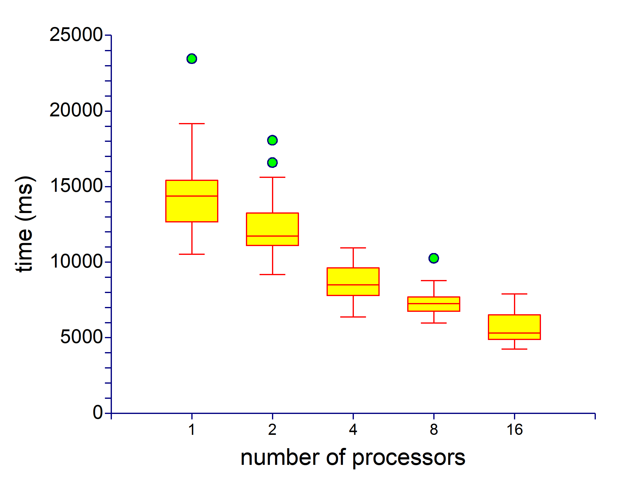
Figure 1. Computing time of b6e6rl for function Griewank, dimension d=50
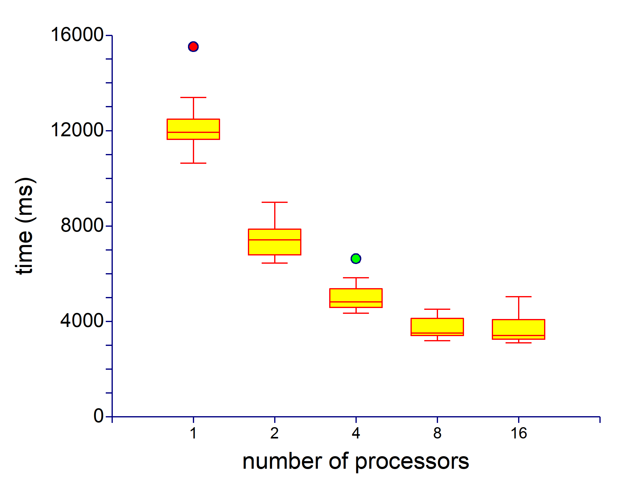
Figure 2. Computing time of b6e6rl for function Schwefel, dimension d=50
References
| [1] | Bäck, T.: Evolutionary algorithms in theory and practice. Oxford University Press, New York (1996). |
| [2] | Brest, J., Greimer, S., Boškovič, B., Mernik, M., Žumer, V.: Self-adapting control parameters in differential evolution: A comparative study on numerical benchmark problems. IEEE Transactions on Evolutionary Computation 10, 646–657 (2006). |
| [3] | Kaelo, P., Ali, M.M.: A numerical study of some modified differential evolution algorithms. European J. Operational Research 169, 1176–1184 (2006). |
| [4] | Mallipeddi, R., Suganthan, P.N., Pan, Q.K., Tasgetiren, M.F.: Differential evolution algorithm with ensemble of parameters and mutation strategies. Applied Soft Computing 11, 1679–1696 (2011) |
| [5] | Neri, F., Tirronen, V.: Recent advances in differential evolution: A survey and experimental analysis. Artificial Intelligence Review 33, 61–106 (2010) |
| [6] | Price, K.V., Storn, R., Lampinen, J.: Differential evolution: A practical approach to global optimization. Springer (2005) |
| [7] | (1, 2) Storn, R., Price, K.V.: Differential evolution - A simple and efficient heuristic for global optimization over continuous spaces. J. Global Optimization 11, 341–359 (1997) |
| [8] | Tvrdík, J.: Competitive differential evolution. In: Matoušek R., Ošmera P. (eds.) MENDEL 2006, 12th International Conference on Soft Computing, 7–12. University of Technology, Brno (2006) |
| [9] | Tvrdík, J.: Adaptation in differential evolution: A numerical comparison. Applied Soft Computing 9, 1149–1155 (2009) |
| [10] | (1, 2) Tvrdík, J.: Self-adaptive variants of differential evolution with exponential crossover. Analele of West University Timisoara, Series Mathematics-Informatics 47, 151–168 (2009). http://www1.osu.cz/~tvrdik/down/global_optimization.html |
| [11] | Tvrdík, J., Křivý, I.: Differential evolution with competing strategies applied to partitional clustering. In: Rutkowski, L., Korytkowski, M., Scherer, R., Tadeusiewicz, R., Zadeh, L.A., and Zurada, J.M. (eds.) Swarm And Evolutionary Computation, Lecture Notes in Computer Science 7269, 136–144 (2012) |
| [12] | Tvrdík, J., Mišík, L., Křivý, I.: Competing heuristics in evolutionary algorithms. In: Sinčák P. et al. (eds.) Proceedings of 2nd Euro-ISCI, Intelligent Technologies - Theory and Applications, 159–166. IOS Press, Amsterdam (2002) |
| [13] | Tvrdík, J., Poláková, R.: Competitive differential evolution applied to CEC 2013 problems. In: IEEE Congress on Evolutionary Computation 2013 Proceedings, 1651–1657 (2013) |
| [14] | (1, 2) Tvrdík, J., Poláková, R., Veselský, J., Bujok, P.: Adaptive variants of differential evolution: Towards control-parameter-free optimizers. In: Zelinka, I., Abraham, A., and Snášel, V. (eds.) Handbook of Optimization, Intellingent Systems Reference Library 38, 423–449. Springer, Heidelberg New York Dordrecht London (2012) |
| [15] | Zaharie, D.: Influence of crossover on the behavior of differential evolution algorithms. Applied Soft Copmputing 9, 1126–1138 (2009) |